8 Solar Energy
8.1 Introduction
The distribution of solar energy incident across the globe is well measured which makes estimations of potential energy generation relatively easy. Insolation is the technical term for the amount of solar energy reaching the earth’s surface. While there are year-to-year small variations due to changes in the intensity of the sun, the earth’s orbit around the sun, and climate, solar data averages are reliable for forecasting solar insolation potential. Figure 8.1 and 8.2 show the solar radiation distribution around thw world and for the US. While there are other factors that will be discussed, these maps make it easy to see where solar potential is highest.
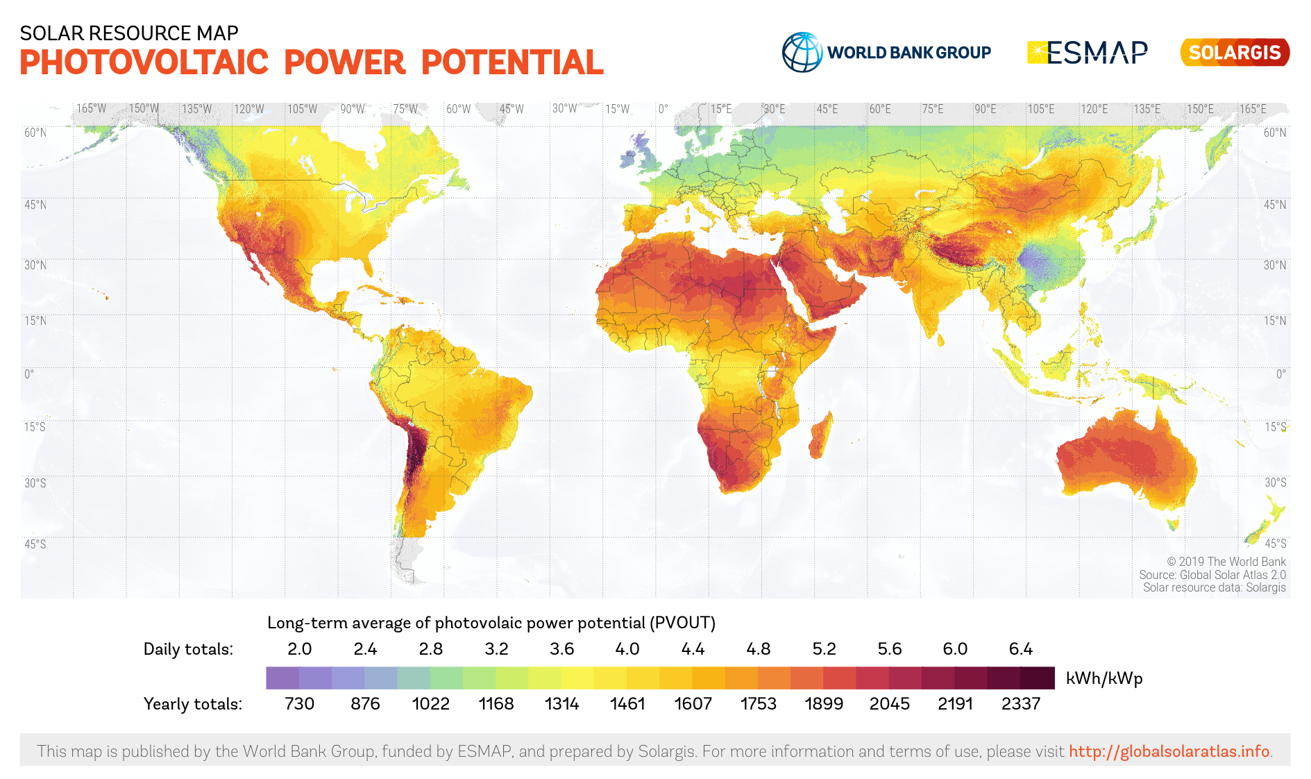
Figure 8.1: Detailed distribution of Solar Insolation across the world . Source: https://solargis.com/maps-and-gis-data/download/world
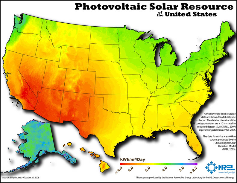
Figure 8.2: Detailed distribution of Average Daily Insolation in the US . Source: https://en.wikipedia.org/wiki/File:NREL_USA_PV_map_lo-res_2008.jpg
Interestingly, the places with the highest solar potential are not always the places where solar PV systems are installed. Figure 8.3 shows US solar power installations which are much more localized than one would expect from the solar potential maps. This is 2017 data, so there are some changes, but still there is something unexpected about this map. Can you think of factors that influence the location of solar systems in this figure?
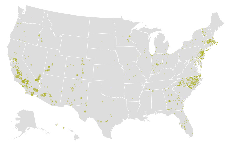
Figure 8.3: Detailed distribution Solar PV Power Plants in the US in 2017. Source: Washington Post, Mapping how the United States generates its electricity, March 2017, https://www.washingtonpost.com/graphics/national/power-plants/
Worldwide, solar energy is increasing across the globe with China leading the way as shown in Figure 8.4. Note that this figure, from Our World in Data website, is plotted on a log scale so China has more installed solar than all of the rest of the countries on this chart combined. This website has a powerful database and interface that allows one to analyze data and add any countries of interest.
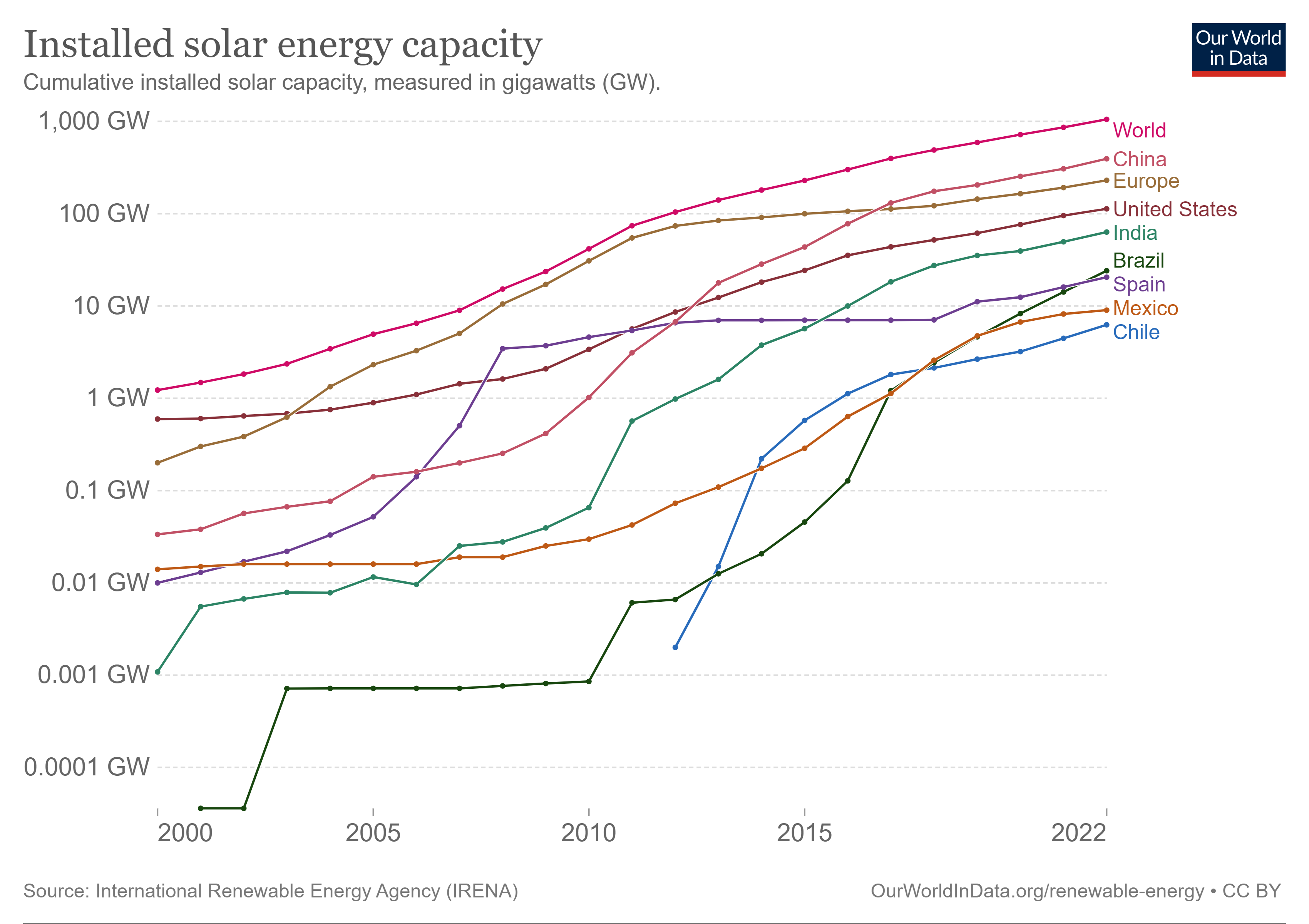
Figure 8.4: Worldwide Installed Solar Capacity. Source: https://ourworldindata.org/grapher/installed-solar-PV-capacity
Unlike fossil fuel power plants in which the fuel is extracted, stored, and transported to the plant where we control its use to generate energy, solar energy availability varies by location, date, and time. As you know from life experience, the sun rises in the east, moves from the horizon to a position high in the sky depending on the seasons, and then sets in the west. Because we understand planetary motion very well, we can predict the sun’s location at any time. This solar motion is shown schematically in Figure 5. Both the altitude and azimuth angles in this figure can be calculated from relatively simple equations found easily (see here for example). From this movement of the sun, south-facing panels (= 0) will produce the most energy on average in most locations. As the orientation of solar panels moves from facing south, the energy is reduced. This reduction is easily quantified so a solar designer can predict energy production for house roofs and other locations which are limited by geometric constraints. The angle of the panels with respect to the ground (= 0) also affects the amount of solar radiation that is incident on a panel.
Many solar panels are installed in a fixed position, for example on a residential house roof with a given pitch, but you can see from Figure 8.5 that more energy could be produced if the panel were moved throughout the day along the axis, with the panel moving from east-facing in the morning through south at midday and to the west in the evening. Similarly, panels could be moved along the xis seasonally with higher angles in the winter when the sun is relatively low above the horizon and lower angles in the summer when the sun is high overhead. For a fixed position, setting qual to the latitude of the location on the globe will generally produce the highest average energy production annually.
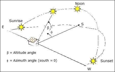
Figure 8.5: Incomings solar energy geometry over the course of a day. Source: J. Randolph and G. Masters, Energy for Sustainability, Island Press, Fig. 7.1, pp. 264, 2008.
While following the sun along 1-axis or 2-axes generates more energy, this comes with the tradeoffs of higher complexity and cost. Tracking systems require energy, motors, gears, and a control system that need maintenance. Generally, tracking systems can payback their extra costs and complexity for large commercial or utility scale projects but not for small residential projects. Solar project developers use solar tracking software to make energy calculations and compare the extra energy generated by tracking along one or two axes compared to the additional costs.
8.2 Basics and Calculations
Solar radiation units are not as straightforward as the energy units for fossil fuels as they are based on the area and angle of the sun’s incidence rather than the mass or volume of solid, liquid, or gas fuels. It is critical for solar calculations to use the proper units.
Irradiance, (wequation (8.1)) also called radiative flux or radiative flux density, is the amount of power radiated through a given area at any instant. The units for irradiance are power per unit area, for example kW m-2. This power is instantaneous and generates energy over time. (E = P x t).
\[\begin{equation} Irradiance = \frac{Power}{Area} \tag{8.1} \end{equation}\]
where power is given in the metric units of W, and area is in m2.
A standard irradiance value is useful for industry to standardize testing conditions since the sun intensity values in different locations. Without such a standard, solar project developers would need to convert panel power ratings based on location. Fortunately, the average irradiance around the world is approximately 1 kW m-2 so this easy to remember benchmark is used as the standard irradiance (Istc) for testing and rating solar panels. Solar panels are exposed to a standard irradiance of 1 kW m-2 of simulated sunlight wavelengths under laboratory conditions to measure the power generated by panels. This leads to a power rating, Prated, for solar panels which is proportional to their surface area. This rated power allows designers and users to make solar energy generation models based on adjustments for their local radiance and conditions compared to the standard irradiance values.
Insolation (short for incident or incoming solar radiation that reaches the earth’s surface) (equation (8.2)) is a related measure of solar radiation energy received on a given surface area over a given time. It is sometimes called solar irradiation or solar irradiation and the units are kWh m-2 as shown in Figure @ref(fig:knitr-InsolationWorld. This value is the solar input, so the output for a solar photovoltaic panel which converts solar radiation into electrical current is given by the insolation multiplied by the area of the panel and its efficiency.
\[\begin{equation} Insolation = \frac{Power \times time}{Area} \tag{8.2} \end{equation}\]
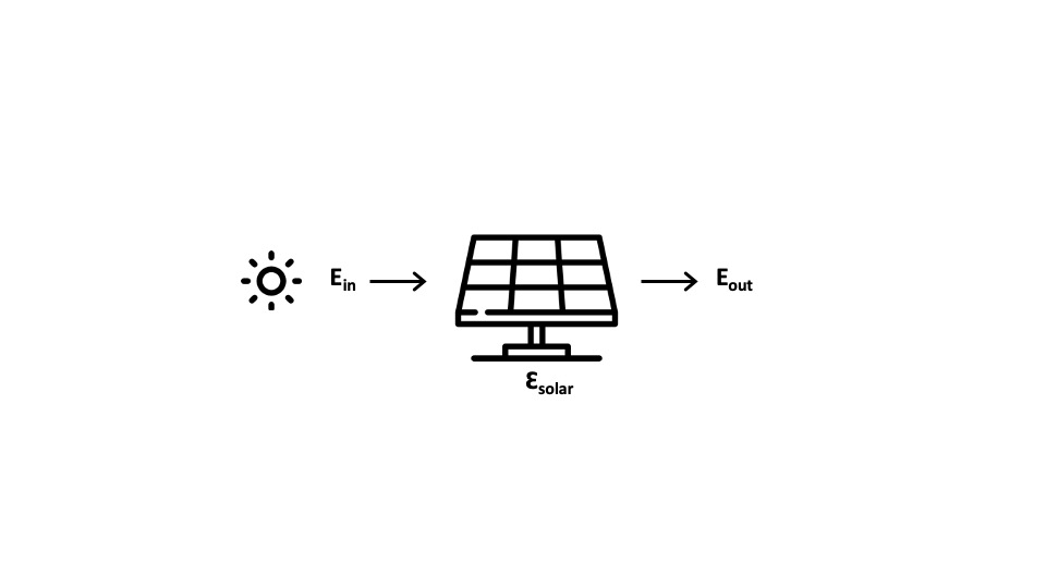
Figure 8.6: Solar diagram representing incoming primary energy from the sun and secondary energy converted to electricity.
Average Daily Insolation (Is) is the insolation averaged over a time period – typically a day (equation (8.3)). Units in this case are kWh m-2 day-1 which can simplify energy calculations further. Figure 8.2uses the metric for the solar color-coding on the US map and these values are easily found for any location in the world. The table below includes the average daily insolation values for south-facing panels in a few US Cities for different tilt angles () and tracking for 1 and 2 axes. Note the variation in the table values for location and tilt angle. Can you explain these variations based on what you have just read?
\[\begin{equation} I_{s}=\frac{Insolation}{RecordingTime} = \frac{Power \times time}{Area \times RecordingTime}=\frac{W \times h}{m^{2} \times day} \tag{8.3} \end{equation}\]
Solar annual average insolation in kWh m-2 day-1 for south-facing surfaces. Adapted from J. Randolph and G. Masters, Energy for Sustainability, Island Press, 2008.
Solar annual average insolation kWh m-2 day-1
| Tilt Angle | Tuscon, AZ | Boulder, CO | Atlanta, GA | Roanoke, VA |
|---|---|---|---|---|
| Horizontal | 5.7 | 4.6 | 4.6 | 4.2 |
| L - 15 | 6.3 | 5.4 | 5.0 | 4.8 |
| Lat | 6.5 | 5.5 | 5.1 | 4.8 |
| 1-Axis (Latitude) | 6.4 | 7.2 | 6.6 | 6.1 |
| 2 - Axis | 9.0 | 7.4 | 6.6 | 6.3 |
Solar photovoltaic panels convert electromagnetic solar energy (photo-) into direct electrical current (-voltaic). It is beyond the scope of this text to explain the physics of solar photovoltaics in detail, but briefly this depends on the electrical properties of materials like silicon (Si), gallium arsenide (GaAs), or cadmium telluride (CdTe). These semiconductors have atomic electron energy levels which do not conduct electricity easily like metals which are conductors. As shown in the simple solar panel schematic of Figure 8.7, current solar photovoltaic (PV) panels depend on multi-layer semiconductors in which an n-type material which has additional electrons is paired with p-type material with missing electrons. Solar PV panels also have metallic conductors on the front surface and an anti-reflective glass protective plate to maximize the sunlight that reaches the semiconductors while being transparent, strong and durable over their 20+ year lifetime.
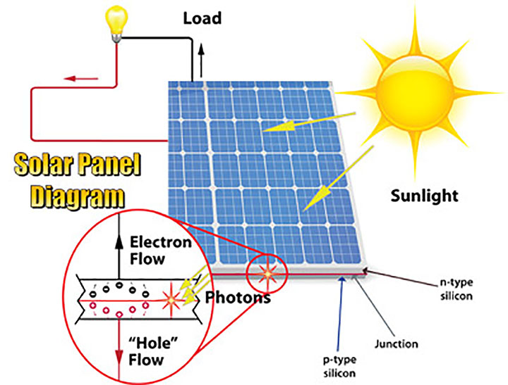
Figure 8.7: Solar Photovoltaic Schematic . Source: https://etap.com/renewable-energy/photovoltaic-array-fundamentals
The efficiency of semiconductors to convert solar radiation (photons) to electrical current depends on the detailed composition, electronic structure, and physics of the materials in the panels. This efficiency is still defined as the output energy (electricity) divided by input energy (incident sunlight). Material scientists, chemists, physicists, and electrical engineers are continually developing new materials for photovoltaic systems. In the research lab, these efficiencies are approaching 50% while in current practice solar photovoltaics that are commercialized have efficiencies around 20%. As efficiencies increase, more electricity is generated from less area given the same incident sunlight. Figure 8.8 from the National Renewable Energy Research Lab (NREL) shows the historical trend for different solar photovoltaic materials over the past few decades.
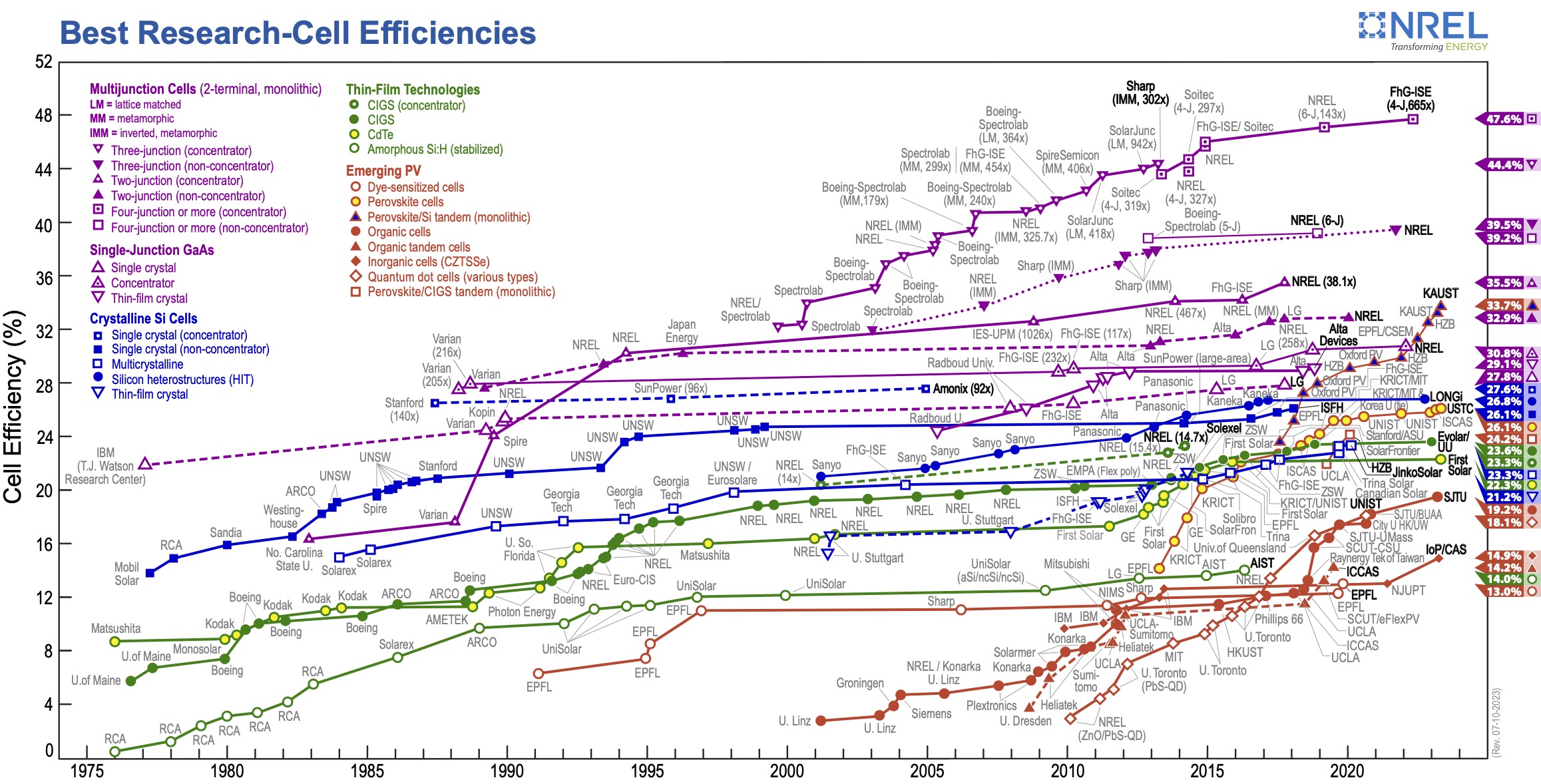
Figure 8.8: Solar Photovoltaic Research Efficiencies from 1975 through th 2023. Source: https://www.nrel.gov/pv/cell-efficiency.html
Solar PV panels generate direct current from the electrons flowing in the circuit due to the photoelectric effect explained above. This direct (DC) current is converted to alternating (AC) current by an inverter to match the electric grid. Off-grid solar installations can use DC current without conversion, for example for a boat or cabin in the woods, but then all the appliances and equipment must also be designed for DC current. Inverter efficiencies have increased in recent years and are now 95% or higher. Additional efficiency losses in solar PV systems includes the wiring, connections, panel degradation, and more factors wwhich can be bundled together for simple energy estimates into a single __ derating factor (DF)__ which is typically on the order of 75 – 85%. A more accurate DF is given by the multiplication of all efficiency losses together. In full solar PV design, more sophisticated software models allow for the modeling of the individual efficiency losses for dozens of factors. An example of a more sophisticated software which is available online is PVWatts from NREL if you are interested in playing around with the parameters to see their effects on solar energy generation.
The simple equation that we will use in this class to quickly estimate solar PV energy generation is shown in Figure 8.9 and equation (8.4). Translated to words, the energy generated in a year is estimated by the number of Panels multiplied by the Rated DC Power per Panel multiplied by the Derating Factor multiplied by the Average Solar insolation divided by the Standard Irradiance and then multiplied by Time. Energy generation for a different time unit is easily calculated simply by changing the time variable. Unit analysis is helpful in this case: kWh yr-1 = Panels x (kW/panel) x (%) x (kWh m-2 day-1) / (1 kW m-2) x (days/yr). Note that to make these units cancel out properly, tannual must be in units of days/year. This equation provides a quick and good estimate of energy production for solar panels without the need for a solar PV modeling program.
\[\begin{equation} E_{annual}= n \times W_{p} \times DF \times \frac{I_{s}}{I_{STC}} \times t_{annual} \tag{8.4} \end{equation}\]
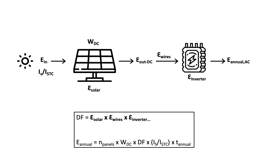
Figure 8.9: Solar diagram and equation representing the conversion of incoming energy (insolation) to usable energy.
As mentioned earlier, the DC panel power is measured by the panel manufacturer and this power rating is published in units of Watts (Wdc). This is the power generated at the standard solar irradiance (ISTC) defined as 1 kW m-2. In the equation above, it is easy to forget about including (ISTC) since the factor of 1 might not seem to make a difference. However, this is problematic as the units will be wrong, which in turn may make you think that you need to include another factor. One way to think about the solar radiation ratio in the equation is that it represents the average number of sun hours at standard conditions. A value of 4.8 hours for this ratio in SW Virginia means that, on average over a year, the total intensity of the sun averaged over a day is equivalent to 4.8 hours at the standard irradiance value of 1 kW m-2. This ratio of actual daily insolation to average global sun insolation in the calculations is much simpler than integrating the sun over the course of a day.
Exercise: Dr. McGinnis’s household solar PV array.
As an example of a recent solar PV project, Dr. McGinnis installed solar panels on his roof in 2022-23. Twenty-seven (27) LG Neon2 Solar Panels with a rating of 360 Wdc were installed on 3 roof sections with different orientations. The total project cost was $2.52/Wdc, not including the available 30% IRA federal tax credit.
To answer the questions below, use an overall derating factor (DF) of 75% due to alignment of 2/3 of the panels away from south, a Roanoke Insolation value of Is = 4.8 kWh/(m2 x day), and a local utility (Appalachian Power Company) electricity cost of $0.16/kWh.
Part 1. How much electricity can this array generate in an average year (kWh/yr)?
Eannual = n x Wp x DF x (IS/ISTC) x tannual
E = (27 x 360 W x (1 kW/1000 W) x 0.75 x (4.8 kWh m-2 day-1 / 1 kW m-2) x 365 days yr-1)
E = 12,772 kWh/yr
Part 2. What is the simple payback time (years)? Recall that payback time was introduced in the previous chapter.
PayBackTime = Ccapitalcost / Sannual
PayBackTime = ($2.52/Wdc x n x Ppanel rating x (1 - credit)) / (Eannual x $0.16/kWh)
PayBackTime = ($2.52/Wdc x 27 x 360 W~ x (1 - 0.3)) / (12,772 kWh x $0.16/kWh)
PayBackTime = 8.4 years
Part 3. How much will the household GHG emissions be reduced per year (tons CO2/yr) if the utility electricity carbon emissions are 1.50 lb CO2/kWh (ignore solar array lifecycle emissions for extraction, manufacturing, transportation and installation)?
CO2 grid = ECgrid x Eproduced
CO2 grid = 1.50 lb CO2/kWh x 12,772 kWh yr-1 x (1 ton / 2000 lbs)
CO2 grid = 9.6 ton CO2 yr-1
The solar PV energy equation above is generally used for solar energy generation estimates instead of capacity factor equation that was used for fossil fuel power plants. The concept of capacity factor – actual energy produced divided by the PV panel rated energy - still applies for solar PV systems, but is more complicated than for traditional steam power plants. While power plants generally run near their rated power during operation, the power for a solar PV panel depends directly on the amount of light available and varies throughout the day. The capacity factor for solar PV is simply the solar insolation value for a location in kWh/(m2 x day) divided by 24 kWh/(m2 x day), the insolation if the sun were shining 24 hours a day. You can see in Figure 8.10 that capacity factors for solar power plants in the US average 25%, and remember this is based only on availability of sunlight and any maintenance, not the efficiency of the system.
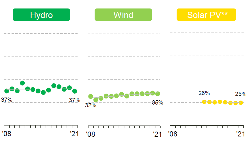
Figure 8.10: Capacity factors for renewable energy facilties. Source: Benchmarking Air Emissions of the 100 Largest Electric Power Producers in the United States Data tables and maps at: www.sustainability.com, September 2022.
Residential houses and commercial buildings can have solar PV that is either off-grid or grid-connected. These options are shown om Figure 8.11 and 8.12. Off-grid systems are not connected to the electrical grid so electricity is only available at the level produced by the available sunlight at any point in time. Batteries are added to store excess electricity not used immediately for later use. Battery systems will be discussed in more detail later, but given battery prices and the reliability of most utility grides, this technology is not yet common for residential housing.
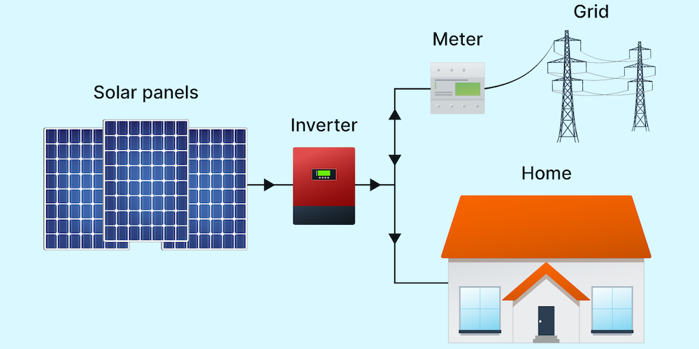
Figure 8.11: Solar Panel Connection Options (top: grid -connected, bottom: off-grid). Source: https://www.solarreviews.com/blog/grid-tied-off-grid-and-hybrid-solar-systems.
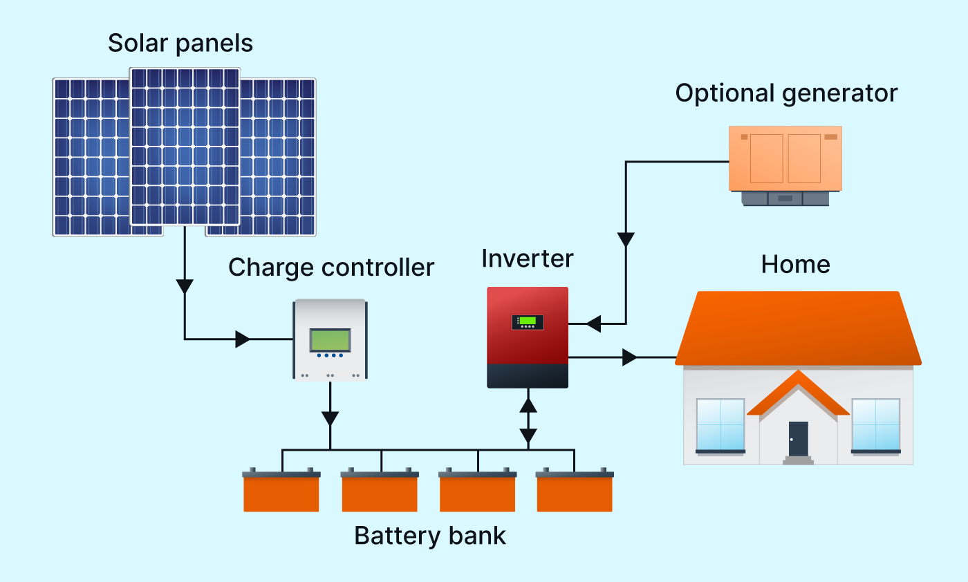
Figure 8.12: Solar Panel Connection Options (top: grid -connected, bottom: off-grid). Source: https://www.solarreviews.com/blog/grid-tied-off-grid-and-hybrid-solar-systems.
Grid-connected system are electrically connected to the existing local utility grid and the building which allows electricity to flow in both directions, to the house when the solar PV is not generating enough electricity to meet current demand or back to the grid when the solar PV system is generating more electricity than is needed. When excess electricity is sent back to the grid, the electric meter runs in reverse, in essence subtracting electricity that you have used from your bill total. Depending on where you live and the utility, electricity sent back to the grid is handled differently. In Virginia, electricity in excess of consumption is considered a credit that can be saved and used later in the year. However, utilities in Virginia also limit the size of residential systems to the approximate annual demand of the house to limit these credits. Some utilities and states offer direct electricity payments instead of credits or electricity payments that vary on the grid demand when the excess electricity is generated.
Batteries can also be added grid-connected systems for a hybrid system which allows more flexibility in controlling electricity flows. In a later chapter, we will discuss these more complex systems in which solar PV panels, batteries, buildings, and electric vehicles are all connected. In such a system, the amount of electricity flowing between these different parts of the system can be controlled at any time using a consumer app.
8.3 Utility Solar
Solar PV flat-panels can be scaled up into much larger arrays for commercial or industrial energy generation. This has the advantage of economies of scale but often requires much more space and infrastructure than for rooftops. Solar PV panels designed over the land, roads, or parking lots have higher costs due to the structures required to support them. There is also often some controversy among different stakeholders when land for solar energy is cleared of forests or replaces agriculture. Nonetheless, these larger arrays are becoming more common as solar panels prices drop with higher production, improved manufacturing and more implementation. Figure 8.13 shows solar panels over a parking area at the Cincinnati Zoo. This type of design also reduces the temperature in the parked cars and sets the stage for electric car charging and integration with the grid as will be discussed in a later chapter.
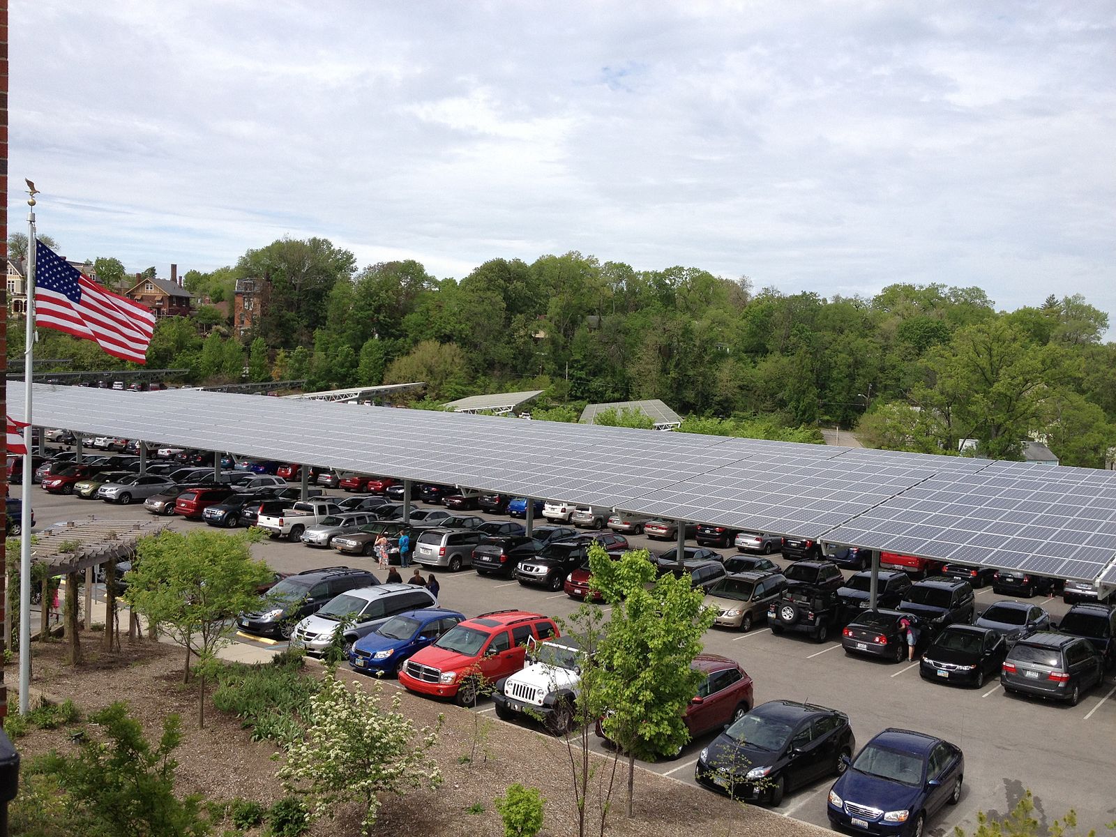
Figure 8.13: Solar panels in a parking lot at the Cincinatti Zoo. Source: https://commons.wikimedia.org/wiki/File:Solar_panels_at_cincinnati_zoo.jpeg
Some flat-panel arrays add 1-axis tracking to follow the sun throughout the day from east to west. A light sensor or computer sun movement model is used with small motors and gears to move the panels orientation throughout the day to maximize the energy generation. As mentioned before, this adds mechanical complexity and cost, but increases the average energy generated as seen in previous table of average daily solar insolation. When implemented properly, this can improve the payback times.
There are other designs that are employed for large utility scale products that will be mentioned briefly here, but not in detail due to the advanced technology. Three of the most common utility-scale technologies are shown in Figure 8.14. Parabolic trough systems use long parabolic reflectors to focus light on oil-filled pipes that run through the focal point of the parabola. These parabolic troughs are controlled to tilt toward the sun for focusing through the day (1-axis tracking). The oil inside of the pipes is heated to temperatures up to 750 {}F which makes steam to run conventional steam turbines and generators. Large parabolic solar arrays with capacities in the 200 – 300 MW range are operational in desert areas of California, Arizona, and Spain.
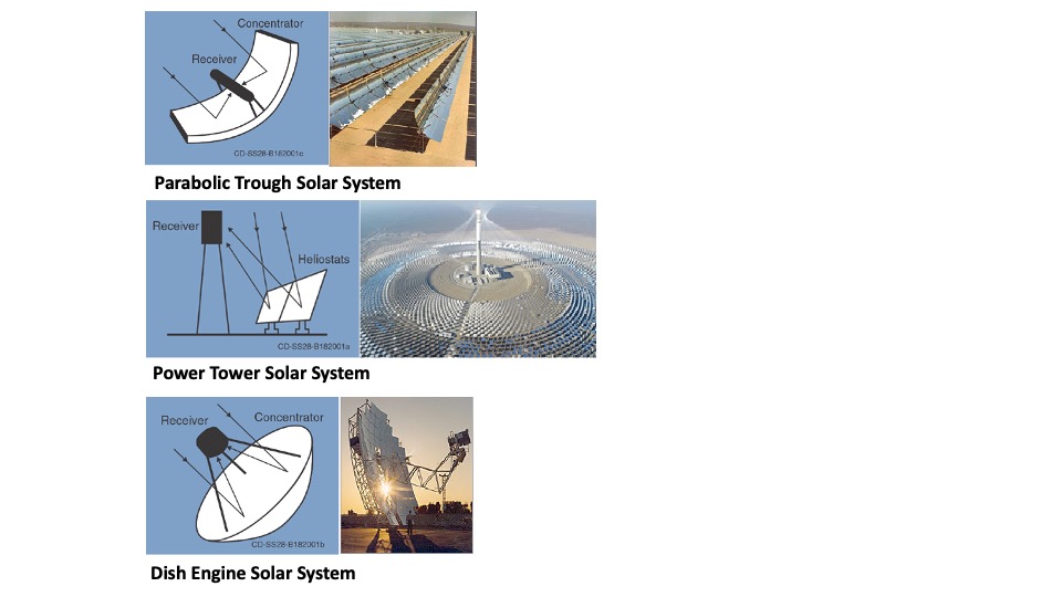
Figure 8.14: Utility Scale Solar Technologies. Source: https://solareis.anl.gov/guide/solar/csp/index.cfm, https://commons.wikimedia.org/wiki/File:50_MW_molten-salt_power_tower_in_hami.jpg#filelinks
Power tower systems use a large array of flat mirrors to track the sun and focus its energy onto a central receiver placed on a tall tower. These systems often have 2-axis tracking to maximize energy collection. The concentrated sunlight heats a fluid, often as molten salt, to temperatures above 1,000 \(^{\circ}\)F. The molten fluid has a high heat capacity and can be used to make steam for electricity generation. Alternatively, since molten salt has a high heat capacity the heat can be stored for days before being converted into electricity. This energy storage acts like a battery and allows the solar energy to be used at night or on days which are cloudy. As an example, the Ashalim solar power tower in Israel has an installed capacity of 121 MW with over 50,000 computer-controller mirrors.
Dish solar heat-engine systems are similar 2-axis trackers but instead use large-mirrored dishes to focus and concentrate sunlight onto a receiver mounted at the focal point of the dish. To capture the maximum amount of solar energy, the dish assembly tracks the sun across the sky. The receiver is integrated into a high-efficiency heat engine, alternatively called a Stirling Engine, with sealed tubes containing gases which expand upon heating and then condense during cool to drive pistons which generate electricity rather than mechanical energy in a combustion engine. Dish systems have smaller capacity, 3 to 25 kW, than the other large-scale systems but have the advantages of being modular and multiple dishes can be connected to create a larger system.
8.4 Solar Heating
While generation of electricity with solar PV panels is what most people think about when solar energy is mentioned, the energy from the sun can also be used for heating. The most common technology for active solar heating is solar water heating. A simple version of this is just a plastic bag of water set out in the sun to heat up for a warm shower later at a campsite, for example. With some added sophistication and technology, this idea turns into active solar hot water heaters as shown schematically in Figure 8.15. Panels, which from a distance look similar to solar PV panels, are placed on the roof and water or heat-transfer fluid is directly heated by absorption of the sunlight. This heated water is connected to a typical hot water heater with a simple pump. The heater water is then stored in an insulated tank for use in household hot water applications. In locations with a high level of solar radiation, the sun can heat water in a hot water heater to temperatures typical of other electric or natural gas water heaters (120 - 140 \(^{\circ}\)F) which eliminates the need for any other heating source. In many locations, the sun is not this intense so backup heating is required over the course of the seasons. However, since the water input to most houses is in the 50 – 60 \(^{\circ}\)F range, any heating of the water from the sun will reduce the overall energy input required to get the hot water temperature up to the setpoint. For example, if 60 \(^{\circ}\)F input water can be heated to 100 \(^{\circ}\)F, approximately 50% less energy is needed to get to a setpoint of 140 \(^{\circ}\)F. Figure 8.16 shows two solar hot water panels on a residential rooftop between the double rows of solar PV panels.
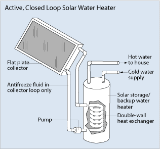
Figure 8.15: Solar heating schematic used on roofs to heat water for domestic use. Source: https://www.energy.gov/energysaver/solar-water-heaters
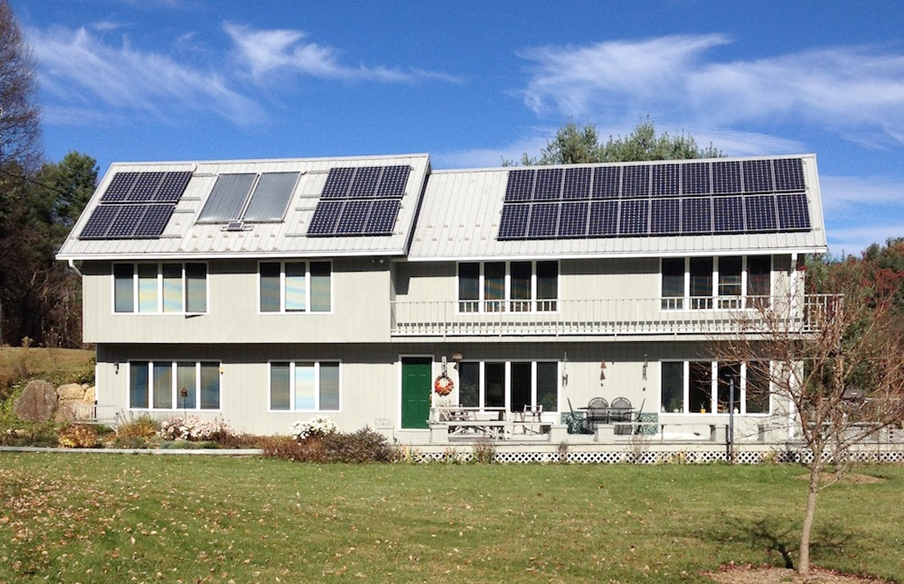
Figure 8.16: A house containing both solar panels and solar heating (larger gray panels). Source: www/solarconnexion.com
There are other types of solar hot water heating, both active and passive. Passive solar heating is also an option for building design as will be discussed in a later chapter on building systems. In these designs, buildings in cold climates are intentionally designed to absorb heat in the building materials such as the floors and the walls during the daylight hours and then slowly release this heat gain once the sun goes down and temperatures drop. This saves energy from other sources for heating of the building space.
The global warming crisis seems insurmountable at times. While there are approaches we’ve discussed regarding how to reduce carbon emissions, understanding the range of options available at this time can provide us with some hope. In fact, many of the technologies are in place already. For example, in the last chapter was an exercise looking at Carbon Capture and Storage (CCS). The objective was to estimate the reduction from capturing 90% of the carbon emissions for eight hundred (800) 1000 MW plants.
Let’s take a moment to backtrack and see where this comes from. The Carbon Mitigation Initiative developed an approach to visualize options to mitigate carbon by 8 billion tons of carbon per year by 2050. In their approach, they developed the stabilization wedges = that is 8 approaches that each account for 1 billion tons of carbon per year.
With this setup, read through this short National Geographic article to learn more about the wedges and options in front of us today. Arguably, our society is beginning to pay for the cost of carbon emissions, from the adverse human health impacts to climate-induced disasters (e.g., droughts, floods, forest fires). One of the points made in the article is that while we have the technology, we’ve not been paying the true cost of our collective choices. While we will not answer this directly in this class, it should be noted that some industries have benefited greatly from non-renewable energy and may be less interested in a renewable energy future.